
티스토리 뷰

▶ CNN을 위한 PyTorch 구현
CIFAR-10 데이터셋을 사용하여 CNN을 구현하려고 합니다.
- 10개의 class
- 약 60,000개의 이미지 데이터셋
필요한 라이브러리 import
import numpy as np
import matplotlib.pyplot as plt
import torch
import torch.nn as nn
import torch.nn.functional as F
from torchvision import transforms, datasets
Device 설정 (GPU/CPU)
if torch.cuda.is_available():
    DEVICE = torch.device('cuda')
else:
    DEVICE = torch.device('cpu')
Batch_size와 Epoch 미리 지정
BATCH_SIZE = 32
EPOCHS = 10
train/test 데이터셋 구성
train_dataset = datasets.CIFAR10(root = "../data/CIFAR_10",
                                  train = True,
                                  download = True,
                                  transform = transforms.ToTensor())

test_dataset = datasets.CIFAR10(root = "../data/CIFAR_10",
                                train = False,
                                transform = transforms.ToTensor())
train/test 데이터로더 구성
- 데이터를 학습에 활용할 수 있는 형태로 변형해주는 작업
train_loader = torch.utils.data.DataLoader(dataset=train_dataset,
                                           batch_size=BATCH_SIZE,
                                           shuffle=True)
test_loader = torch.utils.data.DataLoader(dataset=test_dataset,
                                          batch_size=BATCH_SIZE,
                                          shuffle=False)
방금 구성한 데이터로더를 이용하여 train 데이터셋의 size와 type을 살펴보겠습니다.
for (X_train, y_train) in train_loader:
    print('X_train:', X_train.size(), 'type:', X_train.type())
    print('y_train:', y_train.size(), 'type:', y_train.type())
    break
출력된 결과를 살펴보면,
배치 사이즈를 지정한 대로 하나의 mini batch에는 32개의 데이터가 들어가 있고
input 이미지의 size는 32*32인 것을 확인할 수 있었습니다.
데이터 일부를 출력해서 데이터의 형태를 확인해봅시다.
pltsize = 1
plt.figure(figsize=(10 * pltsize, pltsize))

for i in range(10):
    plt.subplot(1, 10, i + 1)
    plt.axis('off')
    plt.imshow(np.transpose(X_train[i], (1, 2, 0)))
    plt.title('Class: ' + str(y_train[i].item()))
728x90
모델 class 정의
- nn.Conv2d(in_channels, out_channels, kernel_size, stride=1, padding=0, ...)
- Convolution 연산을 위한 Layer
- input의 특징을 뽑아 feature map을 만드는 역할
- 컨볼루션 레이어 끝에는 항상 pooling layer가 붙음
- Convolution 연산을 위한 Layer
class CNN(nn.Module):
  def __init__(self):
    super(CNN, self).__init__()
    self.conv1 = nn.Conv2d(in_channels=3, out_channels=8, kernel_size=3, padding=1)
    self.conv2 = nn.Conv2d(in_channels=8, out_channels=16, kernel_size=3, padding=1)
    self.pool = nn.MaxPool2d(kernel_size=2, stride=2)
    self.fc1 = nn.Linear(8*8*16, 64) # flatten
    self.fc2 = nn.Linear(64, 32)
    self.fc3 = nn.Linear(32, 10)

  def forward(self, x):
    # first block
    x = self.conv1(x)
    x = F.relu(x)
    x = self.pool(x)

    # second block
    x = conv2(x)
    x = F.relu(x)
    x = pool(x)

    # fc
    x = x.view(-1, 8*8*16)
    x = self.fc1(x)
    x = F.relu(x)
    x = self.fc2(x)
    x = F.relu(x)
    x = self.fc3(x)
    x = F.log_softmax(x)
    return x
모델 class를 모두 정의해주었으니 이제 변수에 저장해 줍시다.
model = CNN().to(DEVICE)모델이 최종적으로 어떤 layer를 가졌는지를 한번 출력해 봅시다.
print(model)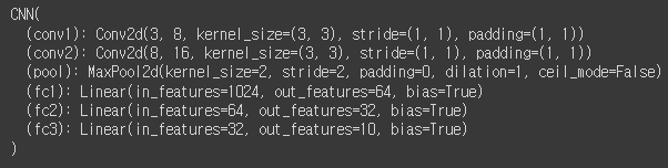
Optimizer, loss 정의
optimizer = torch.optim.Adam(model.parameters(), lr=0.001)
criterrion = nn.CrossEntropyLoss()
train / test 함수 정의
def train(model, train_loader, optimizer, log_interval):
  model.train()
  for batch_idx, (image, label) in enumerate(train_loader):
    image = image.to(DEVICE)
    label = label.to(DEVICE)
    optimizer.zero_grad()
    output = model(image)
    loss = criterion(output, label)
    loss.backward()
    optimizer.step()

    if batch_idx % log_interval == 0:
      print("Train Epoch: {} [{}/{} ({:.0f}%)]\tTrain Loss: {:.6f}".format(
        epoch, batch_idx * len(image),
        len(train_loader.dataset), 100. * batch_idx / len(train_loader),
        loss.item()))
def evaluate(model, test_loader):
model.eval()
test_loss = 0
correct = 0
with torch.no_grad():
for image, laebl in test_loader:
image = image.to(DEVICE)
label = image.to(DEVICE)
output = model(image)
test_loss += criterion(output, label).item()
prediction = output.max(1, keepdim=True)[1]
correct += prediction.eq(label.view_as(prediction)).sum().item()
test_loss /= len(test_loader.dataset)
test_accuracy = 100. * correct / len(test_loader.dataset)
return test_loss, test_accuracy
학습 진행
for epoch in range(1, EPOCHS+1):
  train(model, train_loader, optimizer, log_interval=200)
  test_loss, test_accuracy = evaluate(model, test_loader)
  print("\n[EPOCH: {}], \tTest Loss: {:.4f}, \tTest Accuracy: {:.2f} % \n".format(
        epoch, test_loss, test_accuracy))
...
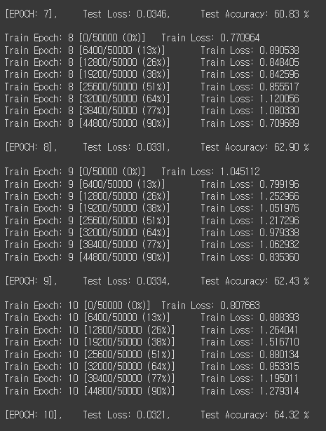
약 64%의 정확도를 보인 것을 확인할 수 있었습니다.
따로 보게 되면 좋은 성능은 아니지만 동일한 데이터셋에 대해서 MLP로 학습을 진행했을 때는 48%의 성능을 보인 것에 비하면 성능이 향상되었다고 볼 수 있었습니다.
728x90
LIST
'빅데이터 인공지능 > 딥러닝' 카테고리의 다른 글
| [딥러닝] RNN(Recurrent Neural Network) (1) | 2022.11.30 |
|---|---|
| [딥러닝] CNN 모델 소개(LeNet, AlexNet, VGG, GoogLeNet, ResNet, DenseNet) (0) | 2022.11.28 |
| [딥러닝] CNN(Convolutional Neural Network) A to Z (1) | 2022.11.26 |
| [딥러닝] MLP를 위한 PyTorch 구현 (0) | 2022.11.26 |
| [딥러닝] ANN을 위한 PyTorch 구현 (1) | 2022.11.26 |
250x250
공지사항
최근에 올라온 글
최근에 달린 댓글
- Total
- Today
- Yesterday
링크
TAG
- 프론트엔드 공부
- rtl
- next.js
- 스타일 컴포넌트 styled-components
- react
- react-query
- 디프만
- 딥러닝
- 자바스크립트 기초
- testing
- 데이터분석
- 리액트 훅
- styled-components
- 프론트엔드
- CSS
- HTML
- 타입스크립트
- 자바
- 파이썬
- 인프런
- 머신러닝
- 프론트엔드 기초
- Python
- 프로젝트 회고
- 자바스크립트
- jest
- 리액트
- JSP
- TypeScript
- frontend
| 일 | 월 | 화 | 수 | 목 | 금 | 토 |
|---|---|---|---|---|---|---|
| 1 | 2 | 3 | ||||
| 4 | 5 | 6 | 7 | 8 | 9 | 10 |
| 11 | 12 | 13 | 14 | 15 | 16 | 17 |
| 18 | 19 | 20 | 21 | 22 | 23 | 24 |
| 25 | 26 | 27 | 28 | 29 | 30 | 31 |
글 보관함